Demo computing and displaying the uncertainty regions

Contents

Loading

Take account of all folders and subfolders of code

init;

% Load the image and the data associated to the files img_1344.*
d=DatasetLoaderToulouse();
imgData = d.getImageDataAtImageName('img_1344');

% Load the polygons of the uncertainty regions
polys = imgData.polys;
% Merge the polygons
mergedPolys = {[],[],[]};
for i=1:3
    mergedPolys{i} = mergePolygons(polys{i});
end

The variable mergedPolys is an cell with the three polygons of the uncertainty regions associated to the three vanishing points. However, theses polygons may be cut by the line at infinity reprented in homoneous coordinate as [0 ; 0 ; 1]. On a 2D projection on the image plane, these polygons would lie on the top and the bottom of the image and would join at infinity. It can be convenient to have the polygons cut by the line at infinity, ie a set of polygons, for example for 2D projection on the image plane. The variable polys provide three sets of polygons (sepatated by the ilne at infinity). Each set of polygons can be merged to get the polygons from mergedPolys.

Compute the uncertainty regions

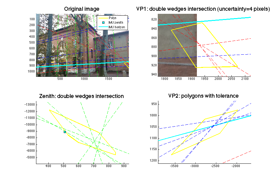
Compute the intersections of the double wedges generated from the three classes of segments. We use an uncertainty of 4 pixels.

polyEstimator = PolyEstimator();
[polys, mergedPolys, maxNoise] = polyEstimator.compute_polys(imgData, 4);

color = ['r', 'g', 'b'];
width = size(imgData.img, 2);
height = size(imgData.img, 1);

% Compute the zenith and the horizon from the IMU data
zenith  = imgData.K * imgData.R_imu * [0 ; 0 ; -1];
zenith  = zenith / zenith(3);
horizon = imgData.Kinv' * imgData.R_imu * [0 ; 0 ; -1];

Plots in the image space

% Store the axes of the 4 subplots in order to simulateneouly draw in the 4 subplots
figure('position', [0, 0, 900, 600]);
axes = [];
for i=1:4
    axes(i) = subplot(2, 2, i);
end

% "Hold on" on the 4 subplots
mhold(axes, 'on');
% Display the image in the 4 subplots
mimagesc(axes, imgData.img);

% Draw the polygons
polygonsLines = [];
for i=1:3
    if length(polys{i}) < 1
        continue;
    end
    % Compute the best axis
    polyAxis = bestPolygonsAxis([Inf -Inf Inf -Inf], polys{i});
    dx = polyAxis(2) - polyAxis(1);
    dy = polyAxis(4) - polyAxis(3);
    polyAxis(1) = polyAxis(1) - dx/5;
    polyAxis(2) = polyAxis(2) + dx/5;
    polyAxis(3) = polyAxis(3) - dy/5;
    polyAxis(4) = polyAxis(4) + dy/5;
    axis(axes(i+1), polyAxis);
    % Concatenate the line segments of the polygons in the same polygonsLines matrix
    for iPoly=1:size(polys{i},2)
        poly = infinitePolygonAxisFit(polys{i}{iPoly}, polyAxis);
        poly = poly([1:end,1],:); % Repeat last vertex
        polygonsLines = [polygonsLines poly(:,1:2)' [NaN ; NaN]];
    end
end
mline(axes, 'XData', polygonsLines(1,:), 'YData',polygonsLines(2,:), 'color', 'y', 'LineWidth',2);

% Plot the zenith and the horizon
mplot(axes, zenith(1), zenith(2), 's', 'LineWidth',1, 'MarkerEdgeColor','k', 'MarkerFaceColor', 'c', 'MarkerSize',6);
mhline(axes, horizon, 'color', 'c', 'LineWidth',2);

% Display all the gt lines
for i=1:size(imgData.lines,1)
    mhline(axes, cross([imgData.lines(i,1:2) 1]', [imgData.lines(i,3:4) 1]'), 'LineStyle', '--', 'Color', color(imgData.vp_association(i)));
end

% Set the legend, title and axis
legend(axes(1), {'Polys', 'IMU zenith', 'IMU horizon'});

t = title(axes(1), 'Original image');
set(t, 'FontSize', 18);
t = title(axes(2), sprintf('VP1: double wedges intersection (uncertainty=%d pixels)', maxNoise));
set(t, 'FontSize', 18);
t = title(axes(3), 'Zenith: double wedges intersection');
set(t, 'FontSize', 18);
t = title(axes(4), 'VP2: polygons with tolerance');
set(t, 'FontSize', 18);

for i=1:4
    axis(axes(i), 'ij');
end
axis(axes(1), [1 width 1 height]);

mhold(axes, 'off');

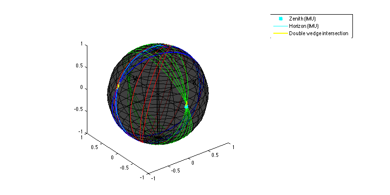
Plot in the Gaussian sphere

figure('position', [0, 0, 800, 400]);
xlim([-1 1]);ylim([-1 1]);zlim([-1 1]);
set(gca,'drawmode','fast');
hold on

% Draw the unit sphere
drawSphere('k');

% Draw the lines
for i=1:size(imgData.lines,1)
    if imgData.vp_association(i) == -1
        continue
    end
    plotCircle3D([0 0 0], (imgData.K' * imgData.linesEq(i,:)')', 1, color(imgData.vp_association(i)));
end

% Draw the horizon and the zenith
phorizon = plotCircle3D([0 0 0], (imgData.K' * horizon)', 1, 'c');
gszenith = imgData.Kinv * zenith;
gszenith = gszenith/norm(gszenith);
pzenith = plot3(gszenith(1), gszenith(2), gszenith(3), 'xc', 'LineWidth',3);

% Draw the intersections of the double wedges
for i=1:3
    mergedPoly = mergedPolys(i);
    gspoly = imgData.Kinv * mergedPoly{1}';
    gspoly = gspoly ./(ones(3,1)*sqrt(sum(gspoly.*gspoly, 1)));
    pPoly = plot3(gspoly(1,[1:end 1]), gspoly(2,[1:end 1]), gspoly(3,[1:end 1]), 'y', 'LineWidth',2);
end
hold off

% Set the title and the legend
t = title(axes(4), 'Gaussian sphere representation');
set(t, 'FontSize', 18);
legend(gca, [pzenith, phorizon, pPoly], 'Zenith (IMU)', 'Horizon (IMU)', 'Double wedge intersection');

Published with MATLAB® R2012b